Plot time curve of average EEG signal with confidence interval

Plot a time course of the average EEG signal amplitude with pointwise confidence intervals (CIs), colour-coded by a user-defined grouping variable such as experimental condition, subject or group. If the condition_column is NULL, all observations are treated as a single condition.

Usage

plot_time_mean(
  data,
  condition_column = NULL,
  FS = 250,
  t0 = 1,
  transp = 0.4,
  y_limits = NULL,
  label_0ms = "stimulus",
  label_offset = c(0, 0),
  legend_title = "Condition"
)

Arguments

data: A data frame, tibble or a database table with input data to plot. It should be an output from compute_mean function or an object with the same structure, containing columns: time with labels of time points and average, ci_low, ci_up with values of average signal and lower and upper CI bounds.
condition_column: Character string specifying the name of the column used to define conditions for plotting. If NULL, all observations are treated as a single condition.
FS: The sampling frequency. Default value is 250 Hz.
t0: Index of the zero time point, i.e. point, where 0 ms should be marked (most often time of the stimulus or time of the response).
transp: A numeric value between 0 and 1 controlling the transparency of the confidence ribbon (corresponding to alpha parameter in geom_ribbon function).
y_limits: A numeric vector of length two, specifying the minimum and maximum y-axis limits. Defaults to NULLfor plot limits determined according to input data.
label_0ms: Character string for the annotation label at the 0ms mark. Default is "stimulus".
label_offset: A numeric vector of length two to offset the stimulus label. The first value indicates a horizontal shift, the second a vertical one. Default is c(0,0) for no shift.
legend_title: Character string specifying the legend title shown in the plot. Default is "Condition". For all observations treated as a single condition (condition_column = NULL) is plotted no legend.

Value

A ggplot object showing the time course of the average EEG signal with pointwise confidence intervals.

Details

The output in the form of a ggplot object allows to easily edit the result image properties.

Examples

# Plot average signal with CI bounds from the sensor E65 excluding outlier epochs (14 and 15)
# for subject 2 - part b) and for the both subjects treated as conditions - part c)

# a) preparing data
# a1) extract required data
edata <- pick_data(epochdata, sensor_rg = c("E65"), epoch_rg = 1:13)
# a2) baseline correction
data_base <- baseline_correction(edata, baseline_range = 1:10)
# a3) average computing
data_mean <- compute_mean(data_base, amplitude = "signal_base", type = "point")

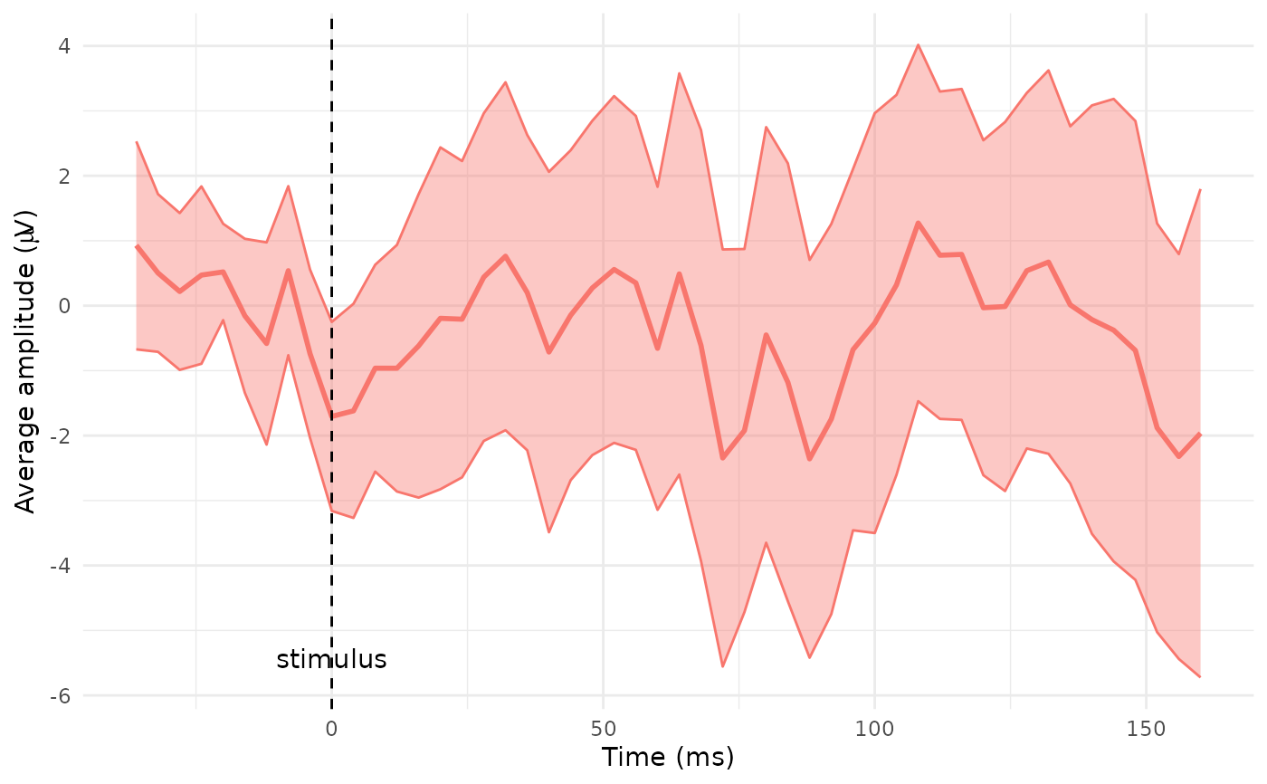
# b) filter subject 2 and plot the average line with default settings
# (the whole dataset treated as one condition, no legend plotted)
data_mean2 <- data_mean |>
dplyr::filter(subject == 2) # or use pick_data(data_mean, subject_rg = 2)
plot_time_mean(data = data_mean2, t0 = 10)


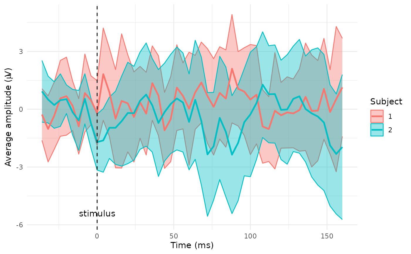
# c) plot the time course by subject (treated as a condition)
plot_time_mean(data = data_mean, condition_column = "subject", t0 = 10, legend_title = "Subject")


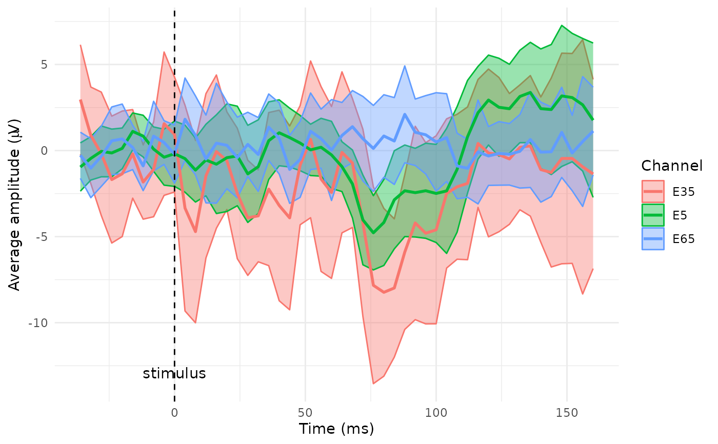
# Plot average signal with CI bounds for subject 1 from three chosen sensors
# preparing data
edata <- pick_data(epochdata, subject_rg = 1, sensor_rg = c("E5", "E35" ,"E65"),
                 epoch_rg = 1:13)
data_base <- baseline_correction(edata, baseline_range = 1:10)
data_mean <- compute_mean(data_base, amplitude = "signal_base", type = "point")
# plot the time course by sensor (channel)
plot_time_mean(data = data_mean, condition_column = "sensor", t0 = 10, legend_title = "Channel")