
Overview
The diegr package enables researchers to visualize high-density electroencephalography (HD-EEG) data with animated and interactive graphics, supporting both exploratory and confirmatory analyses of sensor-level brain signals.
The package diegr includes:
- interactive boxplots (
boxplot_epoch(),boxplot_subject(),boxplot_rt()) - interactive waveforms (
interactive_waveforms()) and surface plots (interactive_surfaceplot(),interactive_surfaceplot_curves()) - topographic maps in 2D (
topo_plot()) - scalp plots in 3D (
scalp_plot()) - functions for computing summary statistics, baseline correction, pointwise and jackknife means (
summary_stats_rt(),baseline_correction(),compute_mean()) - functions for easy selection of data subsets or regions of interest (
pick_data(),pick_region()) - functions for plotting the mean with pointwise confidence intervals (
plot_time_mean(),plot_topo_mean()) - animations of the time course of raw signals or averages in 2D and 3D (
animate_topo(),animate_topo_mean(),animate_scalp())
Installation
You can install the current version of diegr from CRAN with:
install.packages("diegr")or the latest development version from GitHub with:
# install.packages("pak")
pak::pak("gerslovaz/diegr")
Data
Due to the large volumes of data obtained from HD-EEG measurements, the package allows users to work directly with database tables (in addition to common formats such as data frames or tibbles). This approach is much more memory-efficient.
The database you want to use as input to diegr functions must contain columns with the following structure:
-
group- group IDs, -
subject- subject IDs, -
sensor- sensor labels, -
epoch- epoch numbers, -
condition- experimental condition labels, -
time- time-point indices (as sampling indices, not in ms), -
signal- the EEG signal amplitude in microvolts (in most functions, the name of the column containing the amplitude can be customized arbitrarily).
Note: It is not necessary for the data to contain all variables, but if it does, they must be named according to the structure presented above. You can use the check_structure() function, which checks the data structure and prints the inferred hierarchy.
The package includes several example datasets:
-
epochdata: epoched HD-EEG data (anonymized small subset of a large HD-EEG study presented in Madetko-Alster et al., 2025) for two subjects and 204 selected sensors at 50 time points (measured using the EGI HCGSN256 system), -
rtdata: response times (time between stimulus presentation and a button press) from the experiment involving a simple visual motor task (anonymized small subset of a large HD-EEG study presented in Madetko-Alster et al., 2025)
as well as datasets containing sensor position coordinates:
-
HCGSN256: a list with Cartesian coordinates of HD-EEG sensor positions in 3D space on the scalp surface and their projection into 2D space according to the EGI HCGSN256 template, -
biosemi128andbiosemi256: lists with Cartesian coordinates of HD-EEG sensor positions in 3D space on the scalp surface and their projection into 2D space according to the BioSemi system with 128 and 256 electrodes, -
system1005: a list with Cartesian coordinates of HD-EEG sensor positions in 3D space on the scalp surface and their projection into 2D space according to the standard 10-05 system.
For more information about the structure of the built-in data, see the package vignette vignette("diegr", package = "diegr").
Quick examples
Interactive boxplot
This basic example shows how to plot interactive epoch boxplots from a chosen electrode at different time points for one subject:
epochdata |>
  pick_data(subject_rg = 1, sensor_rg = "E65") |>
  boxplot_epoch(amplitude = "signal", time_lim = 10:20)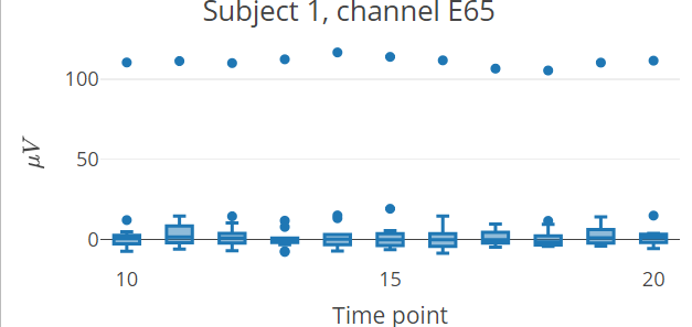
Note: The README format does not support interactive plotly elements, therefore, only a static preview of the result is shown.
Topographic map
data("HCGSN256")
# creating a mesh
M1 <- point_mesh(dimension = 2, n = 30000, type = "polygon",
                 template = "HCGSN256",
                 sensor_select = unique(epochdata$sensor))
# filtering a subset of data to display
data_short <- epochdata |>
  pick_data(subject_rg = 1, time_rg = 15, epoch_rg = 10)
# or you can use dplyr::filter()
# dplyr::filter(subject == 1 & epoch == 10 & time == 15)
# function for displaying a topographic map of the chosen signal on the created mesh M1
topo_plot(data_short, amplitude = "signal", mesh = M1)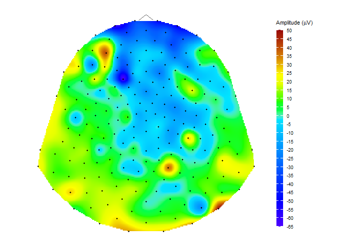
Computing and displaying the average in the time domain
Compute the average signal for subject 2 from channels E65 and E34 (excluding the outlier epochs 14 and 15) and then display it along with confidence interval (CI) bounds (using plot_time_mean() conditioned by sensor).
# extract required data
edata <- epochdata |>
  pick_data(subject_rg = 2, sensor_rg = c("E34", "E65"), epoch_rg = 1:13)
# baseline correction
data_base <- baseline_correction(edata, baseline_range = 1:9)
# compute average
data_mean <- data_base |>
  compute_mean(amplitude = "signal_base", type = "point", domain = "time")
# plot the average line with CI
plot_time_mean(data = data_mean, t0 = 10, condition_column = "sensor", legend_title = "Sensor")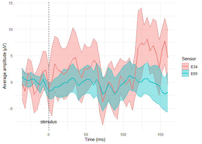
For detailed examples, usage instructions, and troubleshooting information, including system requirements, see the package vignette: vignette("diegr", package = "diegr").
References Madetko-Alster N., Alster P., Lamoš M., Šmahovská L., Boušek T., Rektor I. and Bočková M. The role of the somatosensory cortex in self-paced movement impairment in Parkinson’s disease. Clinical Neurophysiology. 2025, vol. 171, 11-17. https://doi.org/10.1016/j.clinph.2025.01.001
License This package is distributed under the MIT license. See the LICENSE file for details.
Citation Use citation("diegr") to cite this package.